EM-EC | AIMRL

Electromagnetic Field Modeling and Integrated Intelligence for Self-Sensing Autonomous Systems

This research explores the fundamental synergy between electromagnetic fields and computational intelligence to transform mechatronic systems into self-sensing autonomous units. In this domain, we treat the magnetic field not merely as a power source, but as a primary medium for closed-loop control, simultaneously carrying both energy and information.

Motivation and Objective

Magnetic Fields as a Unified Medium: Magnetic fields provide a unique physical medium for both actuation and sensing, enabling non-contact force generation through Lorentz forces and Maxwell stresses. They allow for precise field measurements across multiple non-ferromagnetic media without requiring a line of sight, exhibiting strong robustness to temperature, pressure, and radiation.
Overcoming the Serial-Link Bottleneck: Traditional robotic systems stack multiple single-axis actuators, which introduces mechanical complexity, inertia mismatch, and singular configurations.
Integrated Multi-DOF Objective: Our work seeks to replace discrete serial assemblies with integrated, multi-DOF actuator governed by physics-based models that support state estimation and real-time autonomous control.

The Design Challenge: High-Redundancy Architectures

To illustrate the importance of advanced modeling, we consider a class of multi-DOF actuators characterized by high redundancy. Unlike conventional motors with minimal inputs, these systems employ a large number of distributed stator coils relative to their degrees of freedom. Such architecture provides several critical advantages for autonomous systems:

Efficient heat dissipation: Thermal loads are spread across a high number of stator poles, preventing localized hotspots.
Multi-objective optimization: Redundant inputs enable real-time optimization to minimize use and reduction of bearing reactions via controlled magnetic force distribution.
System resilience: Operation can be maintained even under partial coil failure.

Analyzing and optimizing these complex structures motivated the development of a progressive modeling framework moving from conceptual feasibility to physics-based design and real-time estimation.

Establishing the Principle and Theory: The Forward-Inverse Pairing

The cost-effective design and accurate motion control of integrated actuators with embedded sensors require a bidirectional mathematical framework:

Forward model: Used to predict magnetic fields and actuator behavior for design analysis and optimization.
Inverse solution: Used to estimate position and orientation from measured fields in real-time to support closed-loop control.

While forward models support design, the inverse problem remains challenging because field measurements are often non-unique. Specifically, a single set of sensor measurements may correspond to multiple possible solutions (positions or orientations), requiring complex algorithms to resolve this ambiguity in real-time.

This forward–inverse pairing forms the backbone of integrated actuator–sensor design, where prediction supports design and estimation supports control.

Evolution of Field-Based Modeling Frameworks (Early Works)

To bridge the gap between initial concept and autonomous realization, our early works employ two classes of formulation sequentially:

1. The Energy Method using Field-based Permeance-Model (Lee & Kwan, 1991)

Built on the principle of conservation of energy, this method is a rigorous lumped-parameter approach that captures the essential interplay between electrical input, magnetic storage, and mechanical output.

Fringe and Leakage Effects: It utilizes field-based permeance models to account for energy losses due to magnetic leakage and fringe effects.
Physics of Operation: By applying the principle of virtual work, this approach clarified the physical mechanism of multi-DOF torque generation through the redistribution of magnetic energy stored in the air gaps.
Dynamic Control: The resulting torque-current relationship provided the first deterministic framework for system characterization and motion control.

2.Mathematical Field Formulation (Laplace’s Equation)

Once energy-based feasibility was established, we solved the Laplace’s equation for the magnetic scalar potential to evaluate specific designs with increasing geometric fidelity.

Analytical Solutions (Liang et al., 2006): Separation-of-variables solutions provide physics-transparent models for well-defined geometries.
Finite-Element Analysis (FEA) (Lee, Sosseh & Wei, 2004): Provides high-fidelity modeling of complex geometries and nonlinear materials but is computationally intensive and sensitive to numerical noise, limiting its use in real-time control.
Distributed Multipole (DMP) Modeling (Lee & Son, 2007): Enables fast computation and visualization of field interactions, though limitations arise in extreme near-field regions.

Significance of the Framework

Together, these foundational studies transformed electromagnetic modeling from a purely offline design tool into a bidirectional framework capable of both prediction and perception:

Forward Modeling (Thrust 1): Predict electromagnetic fields efficiently and accurately.
Inverse Sensing (Thrust 2): Recover physical states from measured fields.
Field-based Perception (Thrust 3): Fuse, interpret, and reconstruct physical states for autonomous operation.

Thrust 1: Generalized Distributed Current Source (DCS) Modeling

Thrust 1 establishes fast, physics-based forward models that predict electromagnetic fields and forces for design, optimization, and control. To support parametric analysis of sophisticated designs, we developed the DCS modeling method. This framework shifts from scalar potential to formulating the magnetic vector potential in terms of volume and surface current densities. The DCS method enables the modeling of MFD for permanent magnets (PM), electromagnets (EM), iron plates, and induced eddy currents (EC) in rigorous closed-form.

Computational Efficiency: Enables real-time state reconstruction for autonomous mechatronics.

High-Fidelity Optimization: Delivers the precision necessary for next-generation EM structures.

Environmental Robustness: Maintains accuracy where traditional sensors fail.

The DCS method models electromagnetic systems by discretizing PMs, coils, and ferromagnetic structures into equivalent elemental current sources governed by Maxwell’s equations. Using magnetic vector potentials, these sources enable closed-form evaluation of magnetic fields, forces, and torques with high computational efficiency. As shown in Figure DCS1, the approach integrates source discretization, analytical field formulations, and hierarchical near-field refinement to achieve high accuracy while preserving real-time performance.

Figure DCS1. Distributed Current Source (DCS) Modeling for Closed-Form Analysis of Magneto-Quasi-Static Systems.

Top: Modeling concept and governing formulation.

(a)General 3D geometry of an electromagnetic actuator composed of PM, EM, and ferromagnetic structures.

(b)Discretization into elemental point currents located at the geometric centers of the surface- or volume-sources.

(c)Governing equations for modeling the magneto-quasi-static fields.

Middle: Electromagnetic sources and mathematical representations.(d)Free electric and induced eddy currents

(e)PM sources represented by equivalent magnetizing currents

(f)Magnetic materials modeled through distributed source representations.

Bottom: Magnetic vector potential, MFD, force, and torque equations in closed-form.

(g)MFD of a point current source, including near-source error characteristics.

(h)Octree (or quadtree in 2D) data structure for near-field error correction.

References: Lim and Lee, October 2015; Lim and Lee, December 2015.

A key limitation of point-source representations is reduced accuracy near the source location. As illustrated in (Figure DCS1f, g), the DCS method addresses this by recursively decomposes elemental sources close in the near-field, improving field accuracy with minimal additional computational cost. With sufficient subdivision, the solution converges toward the true field; in practice, the decomposition level is limited to preserve efficiency, and near-source scalar kernels are modified to capture field cancellation within the material geometries.

The DCS method is illustrated through a series of case studies.

1.1 Comparison with Exact Solutions and FEA Simulations

To establish ground truth and evaluate modeling accuracy, the magnetic flux density (MFD) of an axially magnetized circular permanent magnet is derived analytically from the Biot-Savart integral and compared with predictions from DCS and FEA, as summarized in Figure DCS2.

Figure DCS2. Numerical Evaluation of the DCS Modeling Method.

Left: Verification setup, including geometric and material parameters, three DCS discretization schemes (defined by thickness and circumferential divisions), and evaluation metrics based on root-mean-square error (RMSE) and computation time.

Middle: Reference FEA model comprising 151,835 elements, with more than 80% of the tetrahedral mesh devoted to the surrounding air domain.

Right: Comparative results showing magnetic-field predictions from DCS and FEA relative to the analytical solution.

References: Li, Lee, Park & Que (IEEE/ASME AIM2024, 2024).

As revealed in Figure DCS2, a DCS model with as few as 12 elements produces field predictions nearly identical to the analytical solution, with significantly lower RMSE and computation time reduced by approximately two orders of magnitude compared with FEA. The heavy reliance of FEA on meshing large air regions not only increases computational cost and memory demand but also introduces numerical sensitivity.

A key advantage of the DCS framework is that magnetic fields at an observation point are computed directly from equivalent current sources without explicitly meshing surrounding non-ferrous regions (including air). This enables efficient closed-form evaluation with accuracy comparable to high-fidelity numerical methods, making DCS particularly suitable for rapid design iteration and real-time actuator–sensor applications.

1.2 Magnetic Leadscrew (Mag-LS):

Figure MLS1 compares the DCS and FEA modeling of a Mag-LS, consisting of a cylindrical rotor and translator equipped with flexible permanent magnets (FPMs) helically wound around their cylindrical surfaces with pitch l. The rotor and translator magnets possess equal-magnitude radial magnetizations M but opposite polarity, forming a symmetric helical magnetic structure. When an external torque is applied to the rotor, the Mag-LS converts rotary displacement θ into linear motion ζ and an axial force f=.

Figure MLS1 Comparison of DCS and FEA models of a Mag-LS.

（a）Schematics: Geometry and operating principle of the helically magnetized rotor–translator pair.

（b）DCS model: Discretization of the FPMs into equivalent surface current density (SCD) sources derived from the cross product of the circumferential surface normal and radial magnetization vectors. Because no SCD exists on circumferential surfaces, the DCS representation discretizes the remaining four surfaces along thickness, width, and length directions

（c）FEA model: High-fidelity numerical model including free-meshed tetrahedral elements representing the surrounding air domain.

（d）Force prediction: Comparison between DCS-predicted axial force acting on the translator (computed from surface current K interacting with rotor magnetic flux density B) and FEA results (red dots).

References: Li, Lee, Park & Que (IEEE/ASME AIM2024, 2024).

As shown in Figure MLS1(d), the FEA and DCS predictions agree closely in magnitude and trend; however, the FEA results exhibit noticeable numerical noise due to integration over the large meshed air domain, whereas the DCS model provides smooth, closed-form predictions with significantly lower computational cost. This case highlights the suitability of DCS for analyzing and designing field-coupled actuation mechanisms such as magnetic leadscrews.

1.3 Induced Eddy Current Density (ECD): DCS State-Space J-ϕ Formulation

Figure EC1 shows a representative eddy-current system in which a time-varying magnetic field generated by the electromagnet (EM) coil induces ECD within a conductive material while simultaneously magnetizing the medium. Using the DCS framework, the conventional 3D eddy-current boundary-value problem is reformulated in state-space form, converting it into an initial-value problem that directly solves for the current density J under a prescribed input current u.

Figure EC1. EM-Conductor System Modeled using the DCS Method.

(a)Induced ECD: Time-varying magnetic fields from the EM coil. generate eddy currents within the conductive medium.

(b)DCS state formulation: State equation and associated continuity/boundary constraints defined on discretized elemental sources.

(c)Element refinement: Thickness-wise subdivision guided by skin-depth effects to equalize current density distribution across elements.

(d)Aspect-ratio effects: Influence of element geometry on kernel accuracy; approximation error increases as the observation point approaches the source, and convergence improves as element shapes approach a 1:1:1 aspect ratio.

The DCS formulation enables direct analysis of ECD responses under arbitrary current excitation. As demonstrated in Figure EC2, a rectangular pulse input is applied to the EM coil, and the resulting transient MFD is measured to investigate the presence of a hidden rectangular blind hole. The differential signal between defective and defect-free cases is also simulated.

As shown in Figure EC2, the DCS-predicted transient responses closely match the FEA results in both amplitude and temporal evolution. In contrast, the FEA output exhibits noticeable fluctuations arising from numerical discretization and extensive air-domain meshing. These results demonstrate the effectiveness of the DCS framework for dynamic eddy-current analysis and reliable detection of subsurface defects in conductive structures.

Figure EC2. Validation of DCS models for Harmonic and Transient EC Responses.

Top: Harmonic response (2D Axisymmetric DCS Modeling vs. Experiment)

(a)EM–plate Configuration: The EC system consists of a 60-turn coil and an austenitic 304L stainless-steel plate. While nominally nonmagnetic, the plate may exhibit weak magnetization (μr 1.08) due to cold work.

(b)Magnitude Response: DCS predictions for both μr=1 and μr=1.08 produce nearly identical magnitude spectra, both of which closely align with experimental measurements.

(c)Phase Response: At low-frequency (f < 1kHz), the phase differs noticeably between the two permeability cases. This demonstrates that the DCS framework can resolve the influence of very small relative permeability on EC-generated MFD—effects often neglected when materials are assumed strictly nonmagnetic.Bottom: Transient response (3D DCS Modeling under Pulsed Current Excitation

(d)Configuration and Excitation: The geometry features a nonmagnetic conductive plate (r=1)with a hidden cavity, driven by a rectangular current pulse in the EM coil.

(e)Time-Domain MFD Response: The transient MFD is measured above the defective conductor to capture the temporal evolution of the field.

(f)Differential Response: The difference between signals from defective and defect-free cases, highlights defect-induced perturbations. This validates the DCS model’s capability for high-fidelity dynamic eddy-current analysis and subsurface flaw detection.

References: Lin, Lee & Hao (IEEE/ASME TMECH, 2018). Hao, Lee & Bai (Journal of Computational Physics, 2020).

1.4 Performance Evaluation and Validation

The effectiveness of the DCS method is demonstrated through its ability to provide computationally efficient, metrically consistent solutions for both static and dynamic electromagnetic systems.

1）Computational Speed and Accuracy vs. FEA

A comparative study using an axially magnetized circular PM established the following:

Efficiency: A DCS model with only 12 elements achieved a computation time of 14.1ms, whereas a comparable FEA model required 3 seconds—a reduction of approximately two orders of magnitude.
Metrological Fidelity: Unlike FEA, which devotes over 80% of its mesh to the surrounding air domain, DCS computes fields directly from current sources, yielding significantly lower Root-Mean-Square Error (RMSE) relative to exact analytical solutions.

2）Structural Modeling of Helical Systems (Mag-LS)

The framework was validated for complex helical magnetic structures, such as the magnetic leadscrew (Mag-LS):

Numerical Stability: DCS-predicted axial forces acting on the translator agreed closely with FEA results in both magnitude and trend.
Noise Suppression: While FEA results exhibited numerical noise due to air-domain discretization, the DCS model provided smooth, closed-form predictions for rapid design iteration.

3）Harmonic and Transient Eddy-Current Analysis

The DCS method extends to time-varying fields, offering superior sensitivity in conductive media analysis:

Permeability Sensitivity: Harmonic analysis demonstrates that the DCS framework can resolve subtle phase shifts caused by very low relative permeability (μr »1.08), which are typically ignored in conventional nonmagnetic assumptions.
Subsurface Defect Detection: Transient response modeling under pulsed excitation accurately identifies perturbations caused by hidden cavities. The DCS-predicted differential signals match FEA results in temporal evolution but avoid the discretization-induced fluctuations inherent in numerical solvers.

Thrust 2: Inverse Field-Based Sensing System

Thrust 2 focuses on non-contact magnetic sensing for multi-DOF motion estimation, designed explicitly for real-time measurement and closed-loop control. Building on the forward field formulations of Thrust 1, this thrust develops inverse magnetic sensing methods that recover position, orientation, and physical states from field measurements in real time.

The central challenge lies in solving inherently nonlinear and often non-unique inverse problems. To address this, we developed complementary sensing paradigms that combine source-based physical modeling with physics-guided Artificial Neural Network (ANN) learning, enabling physically traceable state estimation across a wide spectrum of electromechanical systems.

2.1 Single Magnetic Source and Magnetic Tensor Sensor (MTS):

This section addresses single-source magnetic inversion through a progressive inversion strategy:

Dipole → Physics-guided ANN → Redundant tensor sensing

This progression reflects increasing proximity, complexity, and accuracy requirements, moving from passive geomagnetic detection to high-precision near-field motion estimation.

A. Far-field: Geomagnetic Sensing of Man-Made Objects:

Magnetic tensor sensor (MTS) was developed to localize distant ferrous objects—such as infrastructure components, vehicles, and unexploded ordnance—embedded in the ambient geomagnetic field. In this regime, objects are modeled as magnetic dipoles whose perturbations are superimposed on a largely uniform background field.

Operation Principle: The dipole approximation provides a closed-form, physically interpretable mapping from measured magnetic field gradients (tensor components) to object location.
Robustness: By relying on tensor measurements rather than field magnitude alone, the approach improves robustness to drift, background bias, and orientation variations.
Applications: This passive and non-contact method is well suited for outdoor navigation, environmental monitoring, and safety-critical search applications.

Figure MTS1 illustrates the operating principle and experimental realization of geomagnetic tensor sensing for distant object detection.

Figure MTS1. Magnetic Tensor Sensor for Locating Magnetic Objects in Geomagnetic Field.

Left (Diploe model): A man-made magnetic object is modeled as a dipole perturbing the ambient geomagnetic field localization is inferred from weak field distortions embedded in a large background field.
Middle (Closed-form inverse solution): Spatial derivatives of the magnetic field enable drift -resistant localization and improved robustness relative to magnitude-only sensing.
Right (Sensor Implementation): Experimental demonstrations illustrate outdoor obstacle detection and the role of the orientation-insensitive parameter Q in stabilizing localization.
References: Lee & Li (IEEE TMAG, 2016); Lee, Li & Lin (IEEE/ASME TMECH, 2016)
B. Near-field: Dedicated PM Source for Pose/Location Tracking:
As the object enters the near field, the inverse dipole assumption becomes invalid. To resolve this, we develop a progressive framework that integrates MTS measurements with inverse-field modeling and physics-guided ANN learning.
B.1. Physics-guided MTS/ANN for planar motion estimation

Figure MTS2 illustrates an MTS system for estimating the planar position and orientation of an axially magnetized circular PM attached to the limb. The framework estimates the pose of a dedicated PM relative to the fixed sensor, specifically designed for bed-based rehabilitation monitoring of stroke patients.

Ankle-Joint Kinematics: The system monitors ankle-joint kinematics to help minimize internal joint forces during therapy.
Input Configurations: Guided by the inverse dipole model, two 12-input configurations (ICs) were evaluated: IC1 (Raw MFD) and IC2 (Features derived from the inverse dipole formulation).
Experimental Validation: Both configurations achieve comparable MAE and MSE; however, IC1 requires a deeper hidden-layer structure to reach the performance of IC2, underscoring the value of embedding physical insight into the learning architecture.
Precision Accuracy: Experimental validation confirms an accuracy of approximately 0.23 mm over a 4 mm XZ motion range and 0.06° over a 60° flexion range.

Figure MTS2. MTS/ANN for Human Joint Motion Sensing in the Sagittal Plane.

Top: Schematics illustrating the MTS/ANN sensing framework for planar motion estimation.

(a) MTS configuration and parameters for inverse dipole modeling.

(b) Effects of physics-informed input configurations on ANN- estimation accuracy.

Bottom: Experimental demonstrations of noncontact joint-motion tracing.

(d) Comparison between MTS/ANN-estimated trajectories and video-captured motion.

B.2. Multi-MTS framework for redundant differential measurements

To reduce drift and noise in IMU-based wearables, we designed a multi-MTS system for contactless joint-motion tracking (Figure MTS3.1).

Resolving Ill-Conditioning: Inversion of a single-MTS can become ill-conditioned when the dipole moment is perpendicular to its position. The multi-MTS design employs redundant differential measurements of MFD vectors and gradient-tensor components to overcome this.
Two-Stage Strategy: Estimation is formulated as a two-stage linear least-squares problem involving dipole-based initialization followed by fully-connected ANN refinement to compensate for noise.
Numerical and Experimental Evaluation:

Moving-Sensor Scenarios (Figure MTS3.2): While a single-MTS fails in the presence of an un-calibrated, direction-varying geomagnetic field, the multi-MTS uses differential measurements to eliminate these errors.
ANN Design Trade-offs (Figure MTS3.3, Left) Increasing from three to four hidden layers marginally improves performance at the expense of training time. Accuracy is most effectively enhanced by using statistically representative samples at each measurement point.
Input Sensitivity: Raw input configurations (IC1) can sometimes outperform processed configurations (IC2) because numerical errors introduced by approximating partial derivatives in IC2 can compromise deep learning performance.

Performance: This framework provides unique, stable pose estimates without requiring subtraction of a pre-determined geomagnetic field. It achieves an RMSE of approximately 40 µm in position and 0.1° in orientation—an order-of-magnitude improvement over the single-MTS configuration.

Figure MTS3.1. Differential Magnetic Field/Tensor and Redundant Measurements for Multi-DOF Motion Estimation of a Magnetic Sensing System.

MTS system and MFD sensors.
PM relative to MTS in world XYZ coordinates.
Flowcharts of the two-stage strategy to estimate the position/orientation of the dedicated PM.:
- Single-MTS (12 inputs): (B, G) computed from an average of a 2´2 (S2, S7; S4, S5) array.
- Multi-MTS (27 inputs): (B, G) and four (DB, DG) pairs computed from a 3´3 (S1, …, S9) array.
Prototype multi-MTS and testbed for experimental evaluation.

Figure MTS3.2. Numerical and Experimental Evaluation for Multi-DOF Motion Estimation.

Numerical Evaluation: Comparisons between simulated “measurements” with the references computed from the Biot-Savart’s integral.

(a) Sensor-fixed scenario: Both Single-MTS and Multi-MTS yield the same error performance. However, the multi-MTS uses differential measurements without the need to subtract a pre-calibrated geomagnetic MFD value.

(b) Moving-sensor scenario: Single-MTS (Left) assumes a constant geomagnetic value, resulting in erroneous estimation whereas the multi-MTS (Right) uses different measurements eliminating the direction-varying geomagnetic MFD.

Experimental Validation: Using the prototype and experimental testbed (Figure MTS3.1), the 3 translational and 2 rotational motions in a 3D space are estimated; both the stationary and moving sensor scenarios are considered

(c) In the fixed-MTS scenario, the multi-MTS shows an order smaller RMSE than the Single-MTS which fails in the moving-MTS scenario. The multi-MTS exhibits similar errors in both scenarios, demonstrating that its effectiveness to overcome the limitations of a single-MTS that fails in the presence of an un-calibrated geomagnetic field.

Figure MTS3.3. ANN-Enhanced Multi-MTS for Noise and Model Compensation.

The experimental results illustrate the tradeoffs between the computation efficiency and validation accuracy on the ANN performance, which depends on the number of data (Dn) per location (measurement point) and hidden layers (number of HLs, each with 20 nodes).

Left: An increase from 3 HLs to 4 HLs marginally improves the ANN performance at the expense of training time. The accuracy of the multi-MTS can be effectively enhanced by using statistically representative samples (Ave and ±1, ±2, ±3 SDs) at each location

Right:Both IC1 (27-input, 5-output) and IC2 (32-input, 5-output) yield similar estimation accuracy in the order 500mm. However, IC1 exhibits slightly accurate predictions than IC2; this is because central differences are used to approximate the partial derivatives as inputs, which introduce numerical errors that compromise the deep learning.

References: Jiang & Lee (IEEE/ASME TMECH, 2022); Jiang, Que, Lee & Ji (IEEE Sensors J., 2023)

Research Thrust 2 advances the "integrated intelligence" philosophy by inverting the physics-based field models from Thrust 1 to achieve high-precision state estimation. While single-source systems (MTS) provide foundational localization, the following sections address complex distributed systems where multiple sources and continuous magnetic structures require advanced redundancy and wireless integration to ensure measurement-grade accuracy.

Section 2.2 presents a logical development beginning with redundancy-enabled bijective sensing (MSF1), advancing to multi-DOF orientation estimation within integrated actuator systems (MSF2), and culminating in the implementation of fully embedded actuator–sensor intelligence capable of simultaneous force and displacement estimation (MSF3). Together, these studies demonstrate how inverse field sensing evolves from resolving uniqueness in measurements to enabling real-time, physics-consistent state estimation in autonomous electromechanical systems.

2.2 Multiple Source Multi-Sensor (MSMS) Framework: Uniqueness and Redundancy:

This section advances from single-source inversion (Section 2.1) to multi-source/multi-sensor systems where redundancy becomes the key to uniqueness. In distributed electromagnetic systems, multiple magnetic sources generate overlapping fields that can lead to non-unique solutions. To resolve this, we developed a Multiple-Source Multi-Sensor (MSMS) framework that exploits redundancy in both sensing configuration and field structure, transforming ambiguity into a resource for high-accuracy state estimation.
A. Redundancy for Unique, High-Accuracy Angular Measurement

Figure MSF1 investigates how redundant sensor-placement strategies shape the ANN global-mapping between magnetic measurements and the absolute spin position of a rotor-PM assembly.

Sensor placement and identifiability: Evenly spaced sensors produce identical sinusoidal signals, limiting uniqueness; staggered placement enriches the measurement space through phase-shifted responses.
Feature Exploitation: Variations in sinusoidal magnitude—arising from practical magnetization non-uniformity—serve as discriminative features that support bijective mapping.
Nano-Degree Precision: With staggered placement and sufficient hidden nodes, the ANN mapping achieves an RMSE below 0.1 nano-degrees.

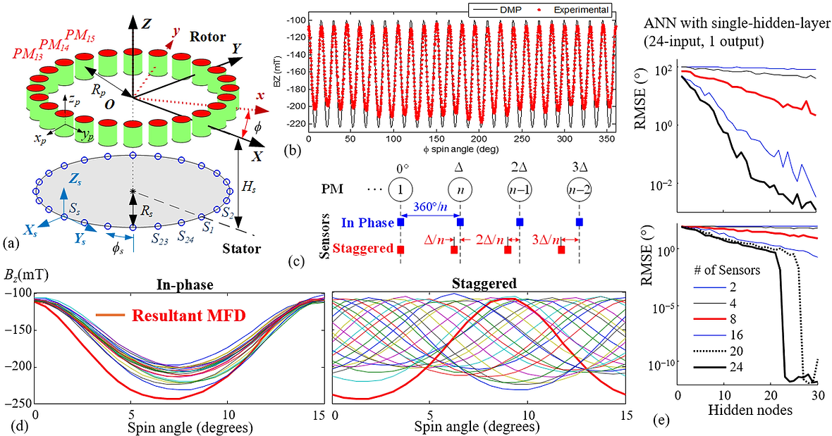
Figure MSF1. MSMS Framework for Highly Accurate Angular Measurement.

(a) Framework: The system measures the axial MFD generated by a 24-PM circular array and establishes a global measurement-to-state mapping through ANN training.
(b) Measurement validation: Phase agreement with the Distributed-Multi-Pole (DMP) model confirms uniform axial magnetization, while systematic variations in sinusoidal magnitude reveal practical non-uniformities in magnetization. These variations act as discriminative features that support a bijective mapping between measurements and angular position.
(c, d) Sensor-placement strategies:
In-phase configuration Evenly spaced sensors produce nearly identical sinusoidal signals, limiting identifiability.
Staggered configuration: Incrementally shifted sensor spacing generates phase-shifted periodic responses that enrich the measurement space and improve uniqueness.
(e) Performance comparison: With staggered placement and sufficient hidden nodes, ANN mapping converges rapidly, achieving RMSE below 0.1 nano-degrees. This behavior is not observed in the in-phase configuration, demonstrating the importance of redundancy and sensor diversity in resolving inverse ambiguity.
These results show that redundancy converts overlapping magnetic fields from a limitation into a resource for ultra-high-precision angular sensing.
References: Foong, Lee & Bai (IEEE/ASME TMECH, 2012).
B. Real-Time Three-DOF Orientation of a Weight-Compensated Spherical Motor
The MSMS framework is extended to a PM-based spherical motor equipped with a Weight-Compensated Regulator (WCR), which both supports the rotor magnetically and houses the sensing architecture.

Figure MSF2. MSMS Framework for three-DOF Orientation Estimation.

(a) Bijective: A one-to-one relationship exists between the spin angle θ and the measurement B(θ) when the WCR rotor-PMs are distinguishable, enabling unique orientation inference.
(b) Non-uniform PM layout: Simulated axial MFD of the rotor PMs during a full rotation at a specified inclination, observed by Sensor S1, illustrating sensitivity to both spin and tilt.
(c) Measurement field structure: Simulated Bz distribution measured by Sensors S1 and S4 across all feasible shaft orientations Z=1 plane, revealing spatial encoding of orientation.
(d) Minimum sensing requirement: T Intersections of three isolines from Sensors (S1, S4, S7) uniquely identify the unit-normal vector ez, demonstrating that three single-axis sensors are sufficient for unique orientation determination.
(e) ANN Implementation and validation: Experimental comparison of three ANN-based sensing configurations. Although three-sensor systems (ANN1, ANN2) ensure uniqueness, sensor placement significantly affects accuracy; ANN2 achieves roughly half the (mean, SD) error of ANN1. The 11-input ANN3 further reduces errors by nearly an order of magnitude, highlighting the value of redundant sensing and higher-dimensional feature mapping for precision orientation estimation.
Figure MSF2 demonstrates how bijectivity, redundancy, and ANN modeling collectively enable stable multi-DOF orientation estimation:

Bijective mapping: Distinguishable rotor PMs create a one-to-one relationship between spin angle and measured magnetic response.
Field encoding of orientation: Spatially structured MFD distributions capture both tilt and spin information.
Minimum sensing requirement: Intersections of isolines from three single-axis sensors uniquely determine the rotor orientation.
Although three sensors ensure uniqueness, sensor placement significantly influences accuracy; increasing redundancy and ANN inputs reduces estimation errors by nearly an order of magnitude.

This study establishes physics-guided redundancy as the foundation for real-time orientation sensing in integrated actuator–sensor systems.
References: Li, Lee, & Hanson (IEEE TIM, 2022).

2.3 Continuous Soft-Magnets: Embedded Wireless Sensing of a Magnetic Leadscrew (Mag-LS)

Section 2.2 resolves non-uniqueness in rigid electromagnetic systems through sensor redundancy and structured field observability. Section 2.3 extends this principle to distributed and deformable magnetic structures, where embedded wireless sensing and physics-guided inference enable simultaneous estimation of displacement and force in real time.
Extending inverse field sensing to distributed and deformable systems, we developed an embedded wireless sensing architecture for magnetic leadscrews and similar mechatronic systems (Figure MSF3). Key capabilities include:

Wireless integration: Embedded magnetic sensing removes cabling constraints in rotating and translating mechanisms.
Simultaneous displacement–force measurement: Physics-based neural networks interpret field deformation to infer both position and interaction force from the same measurements.
Real-time inverse inference: Field-path deviations are reconstructed online, providing physically traceable feedback for manipulation and rehabilitation systems.

Figure MSF3 shows that axial MFD measurements alone yield non-unique displacement solutions; incorporating radial components from multi-axis sensors guarantees uniqueness. A standalone microcontroller integrates multiple neural networks and filters for real-time operation.

Figure MSF3. Wireless Embedded Sensing System with Physics-based ANNs.

(a, b) System architecture: Portable Mag-LS with embedded wireless sensing module housed in the rotor supported by rotary bearings. Five digital three-axis MFD sensors are uniformly arranged on a printed circuit board for distributed field measurement.
(c) Uniqueness of inverse estimation: Simulated axial MFD components (S1, S2, S3) of the translator PM exhibit non-unique axial positions Z when considered alone (top). Incorporating radial components derived from the x and y MFD measurements resolves this ambiguity (bottom), verifying that three or more three-axis sensors guarantee a unique inverse solution.
(d) Wireless ANN implementation: System architecture integrating three independent MSO neural networks for real-time estimation and wireless communication with external devices.
(e) Experimental validation: Translator displacement and axial force are estimated using MSO-NN-z (single-hidden-layer, 40 nodes) and MSO-NN-fz (two hidden-layer, 20 and 15 nodes). The system achieves RMSE/MAE of (0.03, 0.13) mm for displacement and (0.07, 0.33) N for force. Because rotor motion is referenced to a nonstationary frame, deeper learning and larger training datasets are required in addition to signal smoothing from the same MFD measurements.
Experimental results demonstrate RMSE/MAE of approximately (0.03, 0.13) mm for displacement and (0.07, 0.33) N for force, confirming measurement-grade performance in compact embedded systems.
References: Li, Lee, Park & Que (IEEE RAL, 2025).

2.4 Significance of Integrated Inverse Sensing

Research Thrust 2 completes the actuator-sensor loop by providing the sensing counterpart to the forward models of Thrust 1. By combining physics-based modeling, redundancy, and ANN learning, the framework enables:

Metric traceability: Conversion of raw magnetic measurements into stable physical states.
Structural integration: Compact, wireless sensing architectures robust to noise and geometric uncertainty.
Adaptive autonomy: Real-time feedback for intelligent control, rehabilitation, and embedded mechatronic systems.

Together with forward field models (Thrust 1), this inverse framework establishes a closed actuator–sensor loop grounded in first-principles physics.”

Thrust 3: From Estimation to Autonomous Perception

Thrust 3 advances the concept of Integrated Intelligence for autonomous systems by solving complex inverse perception problems under stringent real-time constraints. By combining physics-based models with learning and recursive estimation, this work enables fast, reliable, and interpretable perception for closed-loop operation.

3.1 Sensor Fusion for Full-State Estimation of Multi-DOF Motion

To achieve robust autonomous control of complex mechatronic systems —exemplified by the three-DOF permanent magnet spherical motor (PMSM)—we developed a Kalman filter (KF)-based sensor-fusion framework that treats internal electromagnetic fields as a primary information source.

Dual-Modality Sensing: The system simultaneously measures internal MFD and back electromotive force (back EMF) generated during motion.
Real-Time Full-State Estimation: These complementary signals are fused within a KF framework, to estimate three-DOF angular displacement and angular velocity in real time.
Integrated Intelligence: This architecture eliminates external encoders and leverages the motor's intrinsic electromagnetic fields for physically consistent, closed-loop sensing and control.

Figure SM-SF1 illustrates the embedded sensing architecture, where MFD measurements from the WCR-PMs and back-EMF signals from the stator coils serve as decoupled inputs to the KF-based estimator for full state reconstruction.

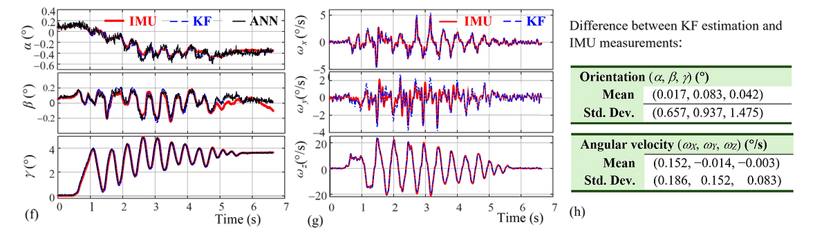
Figure SM-SF1. Embedded Sensor Fusion for Full-State Estimation of a Weight-Compensated Spherical Motor.
(a) Embedded sensing concept using MFD and back-EMF for three-DOF motion estimation.
(b) Physical and measurement models relating rotor orientation and angular velocity to electromagnetic signals.
(c) KF-based fusion framework integrating MFD and back-EMF inputs.
(d, e) Prototype system and experimental setup.
(f-h) Experimental validation by comparing estimated states with IMU and optical data.
Experimental evaluation on a PMSM prototype demonstrates that the field-based sensor-fusion system simultaneously estimates angular displacement and velocity with high accuracy, achieving orientation errors (0.08°mean, 0.06° SD) relative to optical ground truth and (0.16°/s mean, 0.19°/s SD) relative to gyroscope measurements. By combining complementary sensing modalities, the KF framework mitigates both MFD sensor noise and IMU drift, enabling stable and encoder-free full-state estimation for autonomous operation.
While Section 3.1 focuses on full-state motion estimation, the following section extends field-based sensing to material and geometric parameter reconstruction.
Reference: Li, Lee, & Hanson, IEEE Transactions on Instrumentation and Measurement, 2022.

3.2 Magnetic-field based Eddy-Current Sensor for concurrent estimation of geometrical parameters and electrical conductivity

Building on the DCS formulations established in Thrust 1, we exploit EC phenomena to reconstruct hidden physical states and material properties. The resulting framework transforms EC sensing from qualitative inspection into a quantitative measurement modality capable of simultaneously estimating geometric parameters and electrical conductivity.

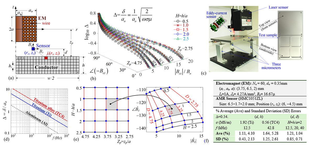
Figure EC3 Simultaneous Estimation of Geometrical Parameters and Electrical Conductivity using Magnetic-Field–Based Eddy-Current Sensing.
(a) CAD model and coordinate definition for the EC sensor, including geometric parameters and governing variables.
(b, d) Material-independent characterization using aluminum (Al), titanium (Ti), and titanium alloy (TC4), demonstrating that responses collapse onto a unified relation when parameterized by normalized skin depth and excitation frequency. Parametric mapping of normalized axial MFD Bcz/Bo (magnitude and phase) as a function of the normalized skin-depth , conductor thickness H and relative sensor location Zp.
(c) Prototype sensor and experimental setup for validating the EC measurement model.
(e) Conceptual mapping between EC-generated MFD (magnitude and phase) and coupled parameters—thickness, relative position, and conductivity.
(f) Experimental results validate the material-independent method to estimate two unknowns out of the three (d, h, ) parameters using a 2D linear interpolation mapping.
Experimental studies conducted over excitation frequencies from 100 Hz to 25 kHz confirm the validity of the material-independent formulation. For a given sensor–conductor configuration, both the magnitude and phase of the EC-induced MFD depend primarily on the normalized skin depth Δ, regardless of material type. This enables simultaneous estimation of conductor thickness, relative location, and electrical conductivity within a unified inverse framework, establishing EC sensing as a measuremetool for process monitoring and material characterization.
References: Lee, Lin, Hao, and Li, IEEE Transactions on Magnetics, 2017.
Moving beyond parameter estimation at a single location, Section 3.3 addresses spatial field reconstruction and defect inspection.

3.3 Magnetic Perception based on Eddy Current for Physical Field Reconstruction

Extending the sensor-fusion and parameter-estimation frameworks of Sections 3.1–3.2, this work advances toward field-based perception—using EC phenomena to reconstruct hidden physical states and detect structural anomalies.
By integrating the harmonic and time-domain DCS formulations from Thrust 1 with inverse modeling and sensing architectures, EC-generated magnetic fields are transformed into quantitative descriptors of material properties, geometry, and defects.
Two complementary problems are addressed:

reconstruction of spatially varying physical fields, and
inspection of defects under static and dynamic conditions.

A. Reconstruction of Nonuniform Electrical Conductivity:
To support in-situ process monitoring and post-fabrication inspection, particularly in metal additive manufacturing and conductive structures, we developed a field-based method for reconstructing spatial variations in electrical conductivity from EC-induced magnetic-field measurements.
Because conductivity cannot be inferred directly from measured MFD signals, the problem is formulated as a two-stage inverse framework. In the first stage, the ECD deviation is estimated using the harmonic DCS model developed in Thrust 1. In the second stage, the reconstructed ECD distribution is recast into a regression problem to recover the spatial conductivity field.

The deviation of eddy-current density (ECD) is first recovered using the harmonic DCS model.
The reconstructed ECD field is then mapped to the underlying conductivity distribution through a regression formulation of the forward model.

Figure EC4 provides sensing architecture and experimental validation. A sensor array replaces conventional single-probe scanning to capture spatial field variations efficiently, while multi-coil excitation mitigates low-sensitivity regions beneath coil centers. The measured and DCS-predicted magnetic-field vectors show strong agreement, validating the physical model.
Reconstructed conductivity maps demonstrate two key outcomes:

Superposition of multi-coil excitations eliminates sensitivity loss near coil centers.
Spatial conductivity fields for plates containing square, rectangular, and circular features are accurately recovered from EC-induced MFD measurements.

The approach is further extended to blind-pocket detection by interpreting local wall thinning as an equivalent conductivity reduction. Experimental results confirm that sensor arrays and multi-coil configurations significantly reduce mechanical scanning requirements while enabling reliable estimation of feature shape and thickness.

Figure EC4 EC-based Magnetic Perception of Non-Uniform Electrical Conductivity.
(a) Experimental Setup: a uniform copper plate and three copper specimens containing square, rectangular and circular features (holes filled with solder). A 5×5 array of two-axis AMR sensors is uniformly distributed on the opposite side of the excitation coil.
(b) EC excitation using either a single annular coil (top) or a multi-coil configuration (bottom) to enhance spatial sensitivity.
(c) Conductivity reconstruction and coil-configuration comparison:
Top row: Comparison between single-coil and multi-coil excitations for a plate with a square feature. The single-coil configuration exhibits reduced sensitivity directly beneath the coil center where the induced ECD is weak, leading to reconstruction artifacts. By superimposing multiple excitation fields, the multi-coil configuration mitigates this low-sensitivity region and produces a more uniform excitation field.
Bottom row: Reconstructed conductivity maps of plates containing square, rectangular, and circular features obtained using the multi-coil excitation. The results demonstrate accurate recovery of feature geometry and thickness variations from measured EC-induced MFD data.
(d) Extension of the method to detect a blind pocket by modeling it as a local wall-thinning region with reduced conductivity.
Reference: Hao, Lee, and Chang, IEEE/ASME Transactions on Mechatronics, 2020.
B. Mechanical High-Speed EC-based Scanning of Cavity Defects:
Building on static field reconstruction, the DCS framework is extended to time-domain EC perception for detecting defects in moving conductors. The transient 3-D EC system is recast into state space and decomposed into defect-free and defect-perturbed subproblems, enabling analysis of defect signatures under varying scanning speeds.
This formulation distinguishes two inspection objectives:

Coarse detection: identifying the presence and approximate location of defects.
Fine detection: estimating defect geometry and size from higher-fidelity transient responses.

Figure EC5 presents the modeling and experimental validation of high-speed EC inspection. The radial component of the EC-induced magnetic field—largely insensitive to motion in defect-free cases—serves as a robust indicator of cavity defects. Its transient envelope converges toward the static response, enabling reliable detection even under rapid scanning.
Speed-dependent error analysis reveals a practical sensing criterion: as normalized scanning speed increases, reconstruction accuracy gradually degrades, transitioning from fine characterization to coarse detection. This provides a physics-based guideline for selecting scanning speeds based on inspection objectives.

Figure EC5. Mechanical Scanning of EC-based Cavity-Defect Detection
(a) Experimental configuration: A 2-D mechanical scanning platform validates high-speed EC inspection of a moving conductor.
(b) Defect-sensitive transient response: The radial (x-axis) component of the EC-induced MFD—relatively insensitive to speed in defect-free cases—serves as a robust indicator of cavity defects. Its envelope converges toward the static case (v0=0), enabling reliable detection under motion.
(c) Speed criteria for detection: Relative-error trends versus normalized scanning speed show that reconstruction accuracy degrades as speed approaches unity. Beyond this threshold, spatial resolution becomes blurred—adequate for coarse detection but insufficient for fine characterization.
The time-domain DCS formulation improves computational efficiency by reducing the solution domain and minimizing experimental calibration. Experimental results confirm that high-speed mechanical scanning can detect cavity defects reliably while maintaining real-time feasibility.
Although demonstrated for surface cavities, the method generalizes to subsurface defect detection. Because EC-generated magnetic fields propagate through non-ferromagnetic media and do not require line-of-sight access, the approach is applicable to non-destructive evaluation, structural health monitoring, and in-situ manufacturing inspection.
References: Guo, Lee, and Xiong, IEEE/ASME Transactions on Mechatronics, 2023.

Selected Publications

Thrust I: Generalized Distributed Current Source (DCS) Modeling

Focus: Establishing physics-based formulations for predicting electromagnetic fields, forces, and dynamic interactions with high computational efficiency.

Lee & Kwan (1991): Introduced a permeance-based energy method that clarifies the mechanism of multi-DOF torque generation and provides a foundational framework for dynamic modeling and control of electromagnetic actuators.
Lee & Son (2007). Developed Distributed Multi-Pole (DMP) modeling to enable fast computation and intuitive visualization of magnetic field interactions in complex actuator–sensor systems.
Lim & Lee (2015): Formulated the DCS method to represent complex electromagnetic structures in closed form, supporting efficient analysis and real-time applications.
Hao, Lee & Bai (2020): Extended DCS modeling to 3D eddy-current systems by recasting boundary-value problems into state-space initial-value formulations, enabling dynamic analysis and transient simulation.

Thrust II:Inverse Solutions & High-Precision Sensing

Focus: Transforming electromagnetic fields from energy carriers into measurement-grade information sources through inverse modeling, redundancy, and physics-guided learning.

Foong, Lee & Bai (2012): Developed a Multiple-Source Multi-Sensor (MSMS) framework that leverages redundancy and staggered sensor placement to resolve inverse ambiguity, enabling bijective mapping and nano-degree angular precision.
Lee & Li (2016): Introduced Magnetic Tensor Sensing (MTS) for drift-resistant localization of distant ferrous objects by exploiting dipole-based inversion of geomagnetic field gradients.
Jiang & Lee (2022): Integrated MTS measurements with physics-guided ANN architectures to achieve stable, non-contact monitoring of limb kinematics, demonstrating measurement-grade accuracy for wearable rehabilitation applications.
Li, Lee, Park & Que (2025): Implemented a fully embedded wireless sensing module that combines multi-axis magnetic measurements with physics-based neural networks to achieve simultaneous force and displacement estimation in magnetic leadscrews

Thrust III: Perception, Sensor Fusion & EC Reconstruction

Focus: Achieving integrated intelligence through physics-based perception, sensor fusion, and inverse field reconstruction for real-time monitoring and inspection.

Lee, Lin, Hao & Li (2017): Established a material-independent inverse framework for eddy-current sensing, enabling measurement-grade characterization of conductive materials across a wide frequency range.
Hao, Lee & Chang (2020): Developed a two-stage inverse formulation to reconstruct spatially varying electrical conductivity and identify hidden geometric features from EC-induced magnetic field measurements.
Li, Lee & Hanson (2022): Implemented a Kalman filter–based sensor fusion scheme that combines internal MFD and back-EMF measurements for real-time full-state estimation of angular displacement and velocity.
Guo, Lee & Xiong (2023): Extended DCS modeling to the time domain, enabling rapid detection and characterization of defects in high-speed moving conductors through transient eddy-current analysis.